Tutorial: Algorithmic Differentiation
Algorithmic differentiation (AD) is also known as automatic differentiation. It is a powerful tool in many fields, especially useful for fast prototyping in machine learning research. Comparing to numerical differentiation which can only provides approximate results, AD can calculates the exact derivative of a given function.
Owl provides both numerical differentiation (in Algodiff.Numerical module) and algorithmic differentiation (in Algodiff.Generic module). In this tutorial, I will only go through AD module since Numerical module is trivial to use.
Algodiff.Generic is a functor which is able to support both float32 and float64 precision AD. However, you do not need to deal with Algodiff.Generic.Make directly since there are already two ready-made modules.
-
Algodiff.Ssupportsfloat32precision; -
Algodiff.Dsupoprtsfloat64precision;
Algodiff has implemented both forward and backward mode of AD. The complete list of APIs can be found in owl_algodiff_generic.mli. The core APIs are listed below.
-
val diff : (t -> t) -> t -> t: calculate derivative forf : scalar -> scalar -
val grad : (t -> t) -> t -> t: calculate gradient forf : vector -> scalar -
val jacobian : (t -> t) -> t -> t: calculate jacobian forf : vector -> vector -
val hessian : (t -> t) -> t -> t: calculate hessian forf : scalar -> scalar -
val laplacian : (t -> t) -> t -> t: calculate laplacian forf : scalar -> scalar
Besides, there are also more helper functions such as jacobianv for calculating jacobian vector product; diff' for calculating both f x and diff f x, and etc.
The following code first defines a function f0, then calculates from the first to the fourth derivative by calling Algodiff.AD.diff function.
open Algodiff.D;;

let map f x = Vec.map (fun a -> a |> pack_flt |> f |> unpack_flt) x;;

(* calculate derivatives of f0 *)
let f0 x = Maths.(tanh x);;
let f1 = diff f0;;
let f2 = diff f1;;
let f3 = diff f2;;
let f4 = diff f3;;

let x = Vec.linspace (-4.) 4. 200;;
let y0 = map f0 x;;
let y1 = map f1 x;;
let y2 = map f2 x;;
let y3 = map f3 x;;
let y4 = map f4 x;;

(* plot the values of all functions *)
let h = Plot.create "plot_021.png" in
Plot.set_foreground_color h 0 0 0;
Plot.set_background_color h 255 255 255;
Plot.plot ~h x y0;
Plot.plot ~h x y1;
Plot.plot ~h x y2;
Plot.plot ~h x y3;
Plot.plot ~h x y4;
Plot.output h;;
Start your utop, then load and open Owl library. Copy and past the code above, the generated figure will look like this.

If you replace f0 in the previous example with the following definition, then you will have another good-looking figure :)
let f0 x = Maths.(
  let y = exp (neg x) in
  (F 1. - y) / (F 1. + y)
);;
As you see, you can just keep calling diff to get higher and higher-order derivatives. E.g., let g = f |> diff |> diff |> diff |> diff will give you the fourth derivative of f.
Gradient descendent (GD) is a popular numerical method for calculating the optimal value for a given function. Often you need to hand craft the derivative of your function f before plugging into gradient descendent algorithm. With Algodiff, derivation can be done easily. The following several lines of code define the skeleton of GD.
open Algodiff.D;;

let gd f x eta epsilon =
  let rec desc xt =
    let g = grad f xt in
    if (unpack_flt g) < (unpack_flt epsilon) then xt
    else desc Maths.(xt - eta * g)
  in
  desc x
;;
Now let's define a function we want to optimise, then plug it into gd function.
let f x = Maths.(sin x + cos x);;

let x_min = gd f (F 0.) (F 0.5) (F 0.00001);;
Because we started searching from 0., the gd function successfully found the local minimum at -2.35619175250552448. You can visually verify that by plotting it out.
let g x = sin x +. cos x in
Plot.plot_fun g (-5.) 5.;;Now let's talk about the hyped neural network. Backpropagation is the core of all neural networks, actually it is just a special case of reverse mode AD. Therefore, we can write up the backpropagation algorithm from scratch easily with the help of Algodiff module.
let backprop nn eta x y =
let t = tag () in
Array.iter (fun l ->
l.w <- make_reverse l.w t;
l.b <- make_reverse l.b t;
) nn.layers;
let loss = Maths.(cross_entropy y (run_network x nn) / (F (Mat.row_num y |> float_of_int))) in
reverse_prop (F 1.) loss;
Array.iter (fun l ->
l.w <- Maths.((primal l.w) - (eta * (adjval l.w))) |> primal;
l.b <- Maths.((primal l.b) - (eta * (adjval l.b))) |> primal;
) nn.layers;
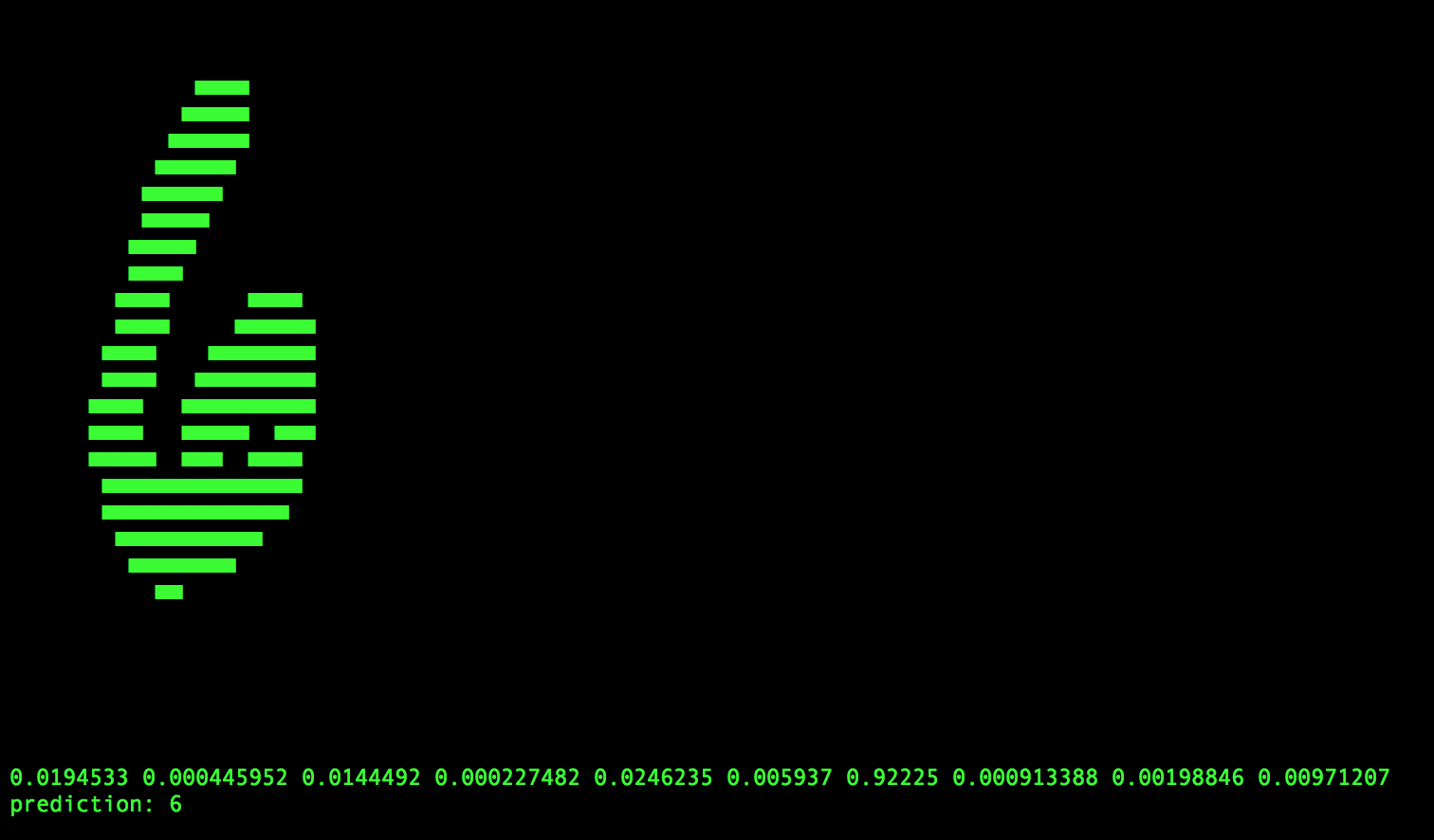
loss |> unpack_fltYes, we just used only 13 lines of code to implement the backpropagation. Actually, with some extra coding, we can make a smart application to recognise handwritten digits. E.g., running the application will give you the following prediction on handwritten digit 6. The code has been included in Owl's example and you can find the complete example in test_mnist.ml
Enjoy Owl! Happy hacking!