scGeneFit

Python code for genetic marker selection using linear programming.

The algorithm is described in https://www.biorxiv.org/content/10.1101/599654v1

Dependencies: numpy, matplotlib, scipy, sklearn.

Examples and source code: https://github.com/solevillar/scGeneFit-python

The package main function is scGeneFit.functions.get_markers()

get_markers(data, labels, num_markers, method='centers', epsilon=1, sampling_rate=1, n_neighbors=3, max_constraints=1000, redundancy=0.01, verbose=True)

• data: Nxd numpy array with point coordinates, N: number of points, d: dimension
• labels: list with labels (N labels, one per point)
• num_markers: target number of markers to select (num_markers<d)
• method: 'centers', 'pairwise', or 'pairwise_centers'
  • 'centers' considers constraints that require that two consecutive classes have their empirical centers separated after projection to the selected markers. According to our numerical experiments is the least general but most efficient and stable set of constraints.
  • 'pairwise' considers constraints that require that points from different classes are separated by a minimal distance after projection to the selected markers. Since all pairwise constraints would typically make the problem computationally too expensive, the constraints are sampled (sampling_rate) and capped (n_neighbors, max_constraints).
  • 'pairwise_centers' after projection to the selected markers every point is required to lie closest to its empirical center than every other class center (sampling and capping also apply here).
• epsilon: constraints will be of the form expr>Delta, where Delta is chosen to be epsilon times the norm of the smallest constraint (default 1) This is the most important parameter in this problem, it determines the scale of the constraints, the rest the rest of the parameters only determine the size of the LP to adapt to limited computational resources. We include a function that finds the optimal value of epsilon given a classifier and a training/test set. We provide an example of the optimization in scGeneFit_functional_groups.ipynb
• sampling_rate: (if method=='pairwise' or 'pairwise_centers') selects constraints from a random sample of proportion sampling_rate (default 1)
• n_neighbors: (if method=='pairwise') chooses the constraints from n_neighbors nearest neighbors (default 3)
• max_constraints: maximum number of constraints to consider (default 1000)
• redundancy: (if method=='centers') in this case not all pairwise constraints are considered but just between centers of consecutive labels plus a random fraction of constraints given by redundancy. If redundancy==1 all constraints between pairs of centers are considered
• verbose: whether it prints information like size of the LP or elapsed time (default True)

from scGeneFit.functions import *

%matplotlib inline
import numpy as np
np.random.seed(0) 

Auxiliary functions

from sklearn.neighbors import NearestCentroid
clf=NearestCentroid()

def performance(X_train, y_train, X_test, y_test, clf):
    clf.fit(X_train, y_train)
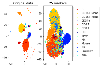
    return clf.score(X_test, y_test)

CITEseq example

Data included in package, from

[1] Marlon Stoeckius, Christoph Hafemeister, William Stephenson, Brian Houck-Loomis, Pratip K Chattopadhyay, Harold Swerdlow, Rahul Satija, and Peter Smibert. Simultaneous epitope and transcriptome measurement insingle cells. Nature Methods, 14(9):865, 2017.

#load data from files
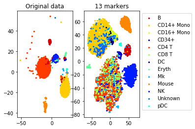
[data, labels, names]= load_example_data("CITEseq")
N,d=data.shape

Use of scGeneFit (center based constraints)

num_markers=25
method='centers'
redundancy=0.25

markers= get_markers(data, labels, num_markers, method=method, redundancy=redundancy)

accuracy=performance(data, labels, data, labels, clf)
accuracy_markers=performance(data[:,markers], labels, data[:,markers], labels, clf)

print("Accuracy (whole data,", d, " markers): ", accuracy)
print("Accuracy (selected", num_markers, "markers)", accuracy_markers)

Solving a linear program with 500 variables and 45 constraints
Time elapsed: 0.3295409679412842 seconds
Accuracy (whole data, 500  markers):  0.8660786816757572
Accuracy (selected 25 markers) 0.7863525588952072

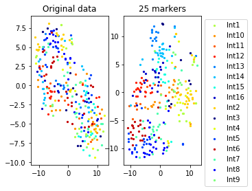
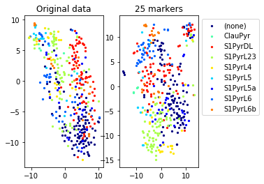
#TSNE plot
a=plot_marker_selection(data, markers, names)

Computing TSNE embedding
Elapsed time: 117.06255102157593 seconds

Use of scGeneFit (pairwise distance constraints)

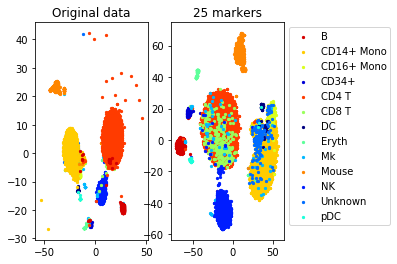
num_markers=25
method='pairwise'
sampling_rate=0.1 #use 10 percent of the data to generate constraints
n_neighbors=3 #3 constraints per point
epsilon=1 #Delta is 10*norm of the smallest constraint
max_constraints=1000 #use at most 1000 constraints (for efficiency)

markers= get_markers(data, labels, num_markers, method=method, sampling_rate=sampling_rate,
                     n_neighbors=n_neighbors, epsilon=epsilon, max_constraints=max_constraints)

accuracy=performance(data, labels, data, labels, clf)
accuracy_markers=performance(data[:,markers], labels, data[:,markers], labels, clf)

print("Accuracy (whole data,", d, " markers): ", accuracy)
print("Accuracy (selected", num_markers, "markers)", accuracy_markers)

Solving a linear program with 500 variables and 1000 constraints
Time elapsed: 6.737841844558716 seconds
Accuracy (whole data, 500  markers):  0.8660786816757572
Accuracy (selected 25 markers) 0.7710340025530927

#TSNE plot
a=plot_marker_selection(data, markers, names)

Computing TSNE embedding
Elapsed time: 118.96086025238037 seconds

Use of scGeneFit (pairwise center based constraints)

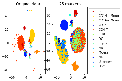
num_markers=25
method='pairwise_centers'
sampling_rate=0.1 #use 10 percent of the data to generate constraints
n_neighbors=0 #neighbors are not used for the center constraints 
epsilon=10 #Delta is 10*norm of the smallest constraint
max_constraints=1000 #use at most 5000 constraints (for efficiency)

markers= get_markers(data, labels, num_markers, method=method, 
                     sampling_rate=sampling_rate, n_neighbors=n_neighbors, epsilon=epsilon, 
                     max_constraints=max_constraints)

accuracy=performance(data, labels, data, labels, clf)
accuracy_markers=performance(data[:,markers], labels, data[:,markers], labels, clf)

print("Accuracy (whole data,", d, " markers): ", accuracy)
print("Accuracy (selected", num_markers, "markers)", accuracy_markers)

Solving a linear program with 500 variables and 1000 constraints
Time elapsed: 4.070271015167236 seconds
Accuracy (whole data, 500  markers):  0.8660786816757572
Accuracy (selected 25 markers) 0.7864686085644655

#TSNE plot
a=plot_marker_selection(data, markers, names)

Computing TSNE embedding
Elapsed time: 118.61988186836243 seconds

One vs all markers

markers2=one_vs_all_selection(data,labels)

accuracy=performance(data, labels, data, labels, clf)
accuracy_markers=performance(data[:,markers2], labels, data[:,markers2], labels, clf)

print("Accuracy (whole data,", d, " markers): ", accuracy)
print("Accuracy (selected", num_markers, "markers)", accuracy_markers)

Accuracy (whole data, 500  markers):  0.8660786816757572
Accuracy (selected 25 markers) 0.7537426018335848

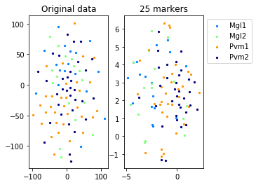
a=plot_marker_selection(data, markers2, names)

Computing TSNE embedding
Elapsed time: 115.60354685783386 seconds

Zeisel example

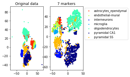
Zeisel data included in package, from

[2] Amit Zeisel, Ana B Munoz-Manchado, Simone Codeluppi, Peter Lonnerberg, Gioele La Manno, Anna Jureus, Sueli Marques, Hermany Munguba, Liqun He, Christer Betsholtz, et al. Cell types in the mouse cortex and hippocampus revealed by single-cell RNA-seq. Science, 347(6226):1138–1142, 2015.

This example exhibits a hierarchical clustering structure. We use the function get_markers_hierarchy that takes the hierarchical structure into consideration to select the constraints.

#load data from file
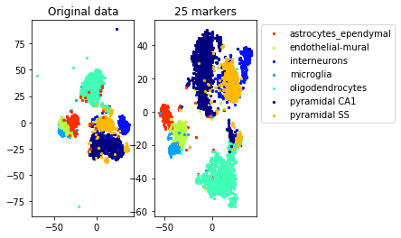
[data, labels, names]=load_example_data("zeisel")
N,d=data.shape

Use of scGeneFit (center based constraints)

num_markers=25
method='centers'
redundancy=0.1

markers= get_markers_hierarchy(data, labels, num_markers, method=method, redundancy=redundancy)

accuracy=performance(data, labels[0], data, labels[0], clf)
accuracy_markers=performance(data[:,markers], labels[0], data[:,markers], labels[0], clf)

print("Accuracy (whole data,", d, " markers): ", accuracy)
print("Accuracy (selected", num_markers, "markers)", accuracy_markers)

Solving a linear program with 4000 variables and 96 constraints
Time elapsed: 67.69524931907654 seconds
Accuracy (whole data, 4000  markers):  0.8745424292845257
Accuracy (selected 25 markers) 0.8861896838602329

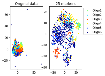
#TSNE plot
a=plot_marker_selection(data, markers, names[0])

Computing TSNE embedding
Elapsed time: 71.29064297676086 seconds

Use of scGeneFit (pairwise distance constraints)

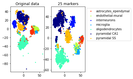
num_markers=25
method='pairwise'
sampling_rate=0.05 #use 5 percent of the data to generate constraints
n_neighbors=3 #3 constraints per point
epsilon=10 #Delta is 10*norm of the smallest constraint
max_constraints=500 #use at most 500 constraints (for efficiency)
use_centers=False #constraints given by pairwise distances

markers= get_markers_hierarchy(data, labels, num_markers, method=method, 
                     sampling_rate=sampling_rate, n_neighbors=n_neighbors, epsilon=epsilon)

accuracy=performance(data, labels[0], data, labels[0], clf)
accuracy_markers=performance(data[:,markers], labels[0], data[:,markers], labels[0], clf)

print("Accuracy (whole data,", d, " markers): ", accuracy)
print("Accuracy (selected", num_markers, "markers)", accuracy_markers)

Solving a linear program with 4000 variables and 1000 constraints
Time elapsed: 40.95984506607056 seconds
Accuracy (whole data, 4000  markers):  0.8745424292845257
Accuracy (selected 25 markers) 0.8435940099833611

Use of scGeneFit (pairwise center based constraints)

num_markers=25
method='pairwise_centers'
sampling_rate=0.05 #use 5 percent of the data to generate constraints
n_neighbors=0 #neighbors are not used for the center constraints
epsilon=10 #Delta is 10*norm of the smallest constraint
max_constraints=500 #use at most 500 constraints (for efficiency)
use_centers=True #constraints given by pairwise distances

markers = get_markers_hierarchy(data, labels, num_markers, method=method, 
                     sampling_rate=sampling_rate, n_neighbors=n_neighbors, epsilon=epsilon)

accuracy=performance(data, labels[0], data, labels[0], clf)
accuracy_markers=performance(data[:,markers], labels[0], data[:,markers], labels[0], clf)

print("Accuracy (whole data,", d, " markers): ", accuracy)
print("Accuracy (selected", num_markers, "markers)", accuracy_markers)

Solving a linear program with 4000 variables and 1000 constraints
Time elapsed: 168.19283509254456 seconds
Accuracy (whole data, 4000  markers):  0.8745424292845257
Accuracy (selected 25 markers) 0.9237936772046589

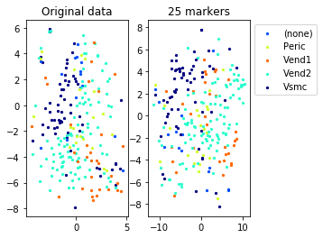
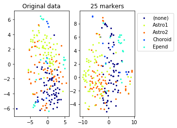
#TSNE plot
a=plot_marker_selection(data, markers, names[0])

Computing TSNE embedding
Elapsed time: 69.88537192344666 seconds

Example from second level of the hierarchy

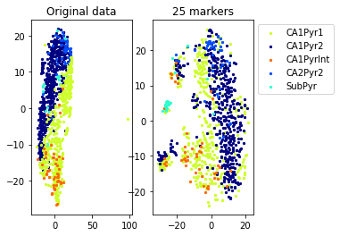
for name in set(names[0]):
    idx=[s for s in range(len(names[0])) if names[0][s]==name]
    aux=plot_marker_selection(data[idx], markers, [names[1][s] for s in idx])

Computing TSNE embedding
Elapsed time: 8.925884008407593 seconds
Computing TSNE embedding
Elapsed time: 1.5634911060333252 seconds
Computing TSNE embedding
Elapsed time: 0.638862133026123 seconds
Computing TSNE embedding
Elapsed time: 7.366800785064697 seconds
Computing TSNE embedding
Elapsed time: 1.0175950527191162 seconds
Computing TSNE embedding
Elapsed time: 2.3961689472198486 seconds
Computing TSNE embedding
Elapsed time: 1.0149860382080078 seconds

One vs all markers

markers2=one_vs_all_selection(data,labels[0])

accuracy=performance(data, labels[0], data, labels[0], clf)
accuracy_markers=performance(data[:,markers2], labels[0], data[:,markers2], labels[0], clf)

print("Accuracy (whole data,", d, " markers): ", accuracy)
print("Accuracy (selected", num_markers, "markers)", accuracy_markers)

Accuracy (whole data, 4000  markers):  0.8745424292845257
Accuracy (selected 25 markers) 0.8569051580698835

a=plot_marker_selection(data, markers2, names[0])

Computing TSNE embedding
Elapsed time: 69.53578591346741 seconds