Python code for genetic marker selection using linear programming.
The algorithm is described in https://www.biorxiv.org/content/10.1101/599654v1
Dependencies: numpy, matplotlib, scipy, sklearn.
Examples and source code: https://github.com/solevillar/scGeneFit-python
The package main function is scGeneFit.functions.get_markers()
get_markers(data, labels, num_markers, method='centers', epsilon=1, sampling_rate=1, n_neighbors=3, max_constraints=1000, redundancy=0.01, verbose=True)
- data: Nxd numpy array with point coordinates, N: number of points, d: dimension
- labels: list with labels (N labels, one per point)
- num_markers: target number of markers to select (num_markers<d)
- method: 'centers', 'pairwise', or 'pairwise_centers'
- 'centers' considers constraints that require that two consecutive classes have their empirical centers separated after projection to the selected markers. According to our numerical experiments is the least general but most efficient and stable set of constraints.
- 'pairwise' considers constraints that require that points from different classes are separated by a minimal distance after projection to the selected markers. Since all pairwise constraints would typically make the problem computationally too expensive, the constraints are sampled (sampling_rate) and capped (n_neighbors, max_constraints).
- 'pairwise_centers' after projection to the selected markers every point is required to lie closest to its empirical center than every other class center (sampling and capping also apply here).
- epsilon: constraints will be of the form expr>Delta, where Delta is chosen to be epsilon times the norm of the smallest constraint (default 1) This is the most important parameter in this problem, it determines the scale of the constraints, the rest the rest of the parameters only determine the size of the LP to adapt to limited computational resources. We include a function that finds the optimal value of epsilon given a classifier and a training/test set. We provide an example of the optimization in scGeneFit_functional_groups.ipynb
- sampling_rate: (if method=='pairwise' or 'pairwise_centers') selects constraints from a random sample of proportion sampling_rate (default 1)
- n_neighbors: (if method=='pairwise') chooses the constraints from n_neighbors nearest neighbors (default 3)
- max_constraints: maximum number of constraints to consider (default 1000)
- redundancy: (if method=='centers') in this case not all pairwise constraints are considered but just between centers of consecutive labels plus a random fraction of constraints given by redundancy. If redundancy==1 all constraints between pairs of centers are considered
- verbose: whether it prints information like size of the LP or elapsed time (default True)
from scGeneFit.functions import *

%matplotlib inline
import numpy as np
np.random.seed(0) from sklearn.neighbors import NearestCentroid
clf=NearestCentroid()
def performance(X_train, y_train, X_test, y_test, clf):
clf.fit(X_train, y_train)
return clf.score(X_test, y_test)Data included in package, from
[1] Marlon Stoeckius, Christoph Hafemeister, William Stephenson, Brian Houck-Loomis, Pratip K Chattopadhyay, Harold Swerdlow, Rahul Satija, and Peter Smibert. Simultaneous epitope and transcriptome measurement insingle cells. Nature Methods, 14(9):865, 2017.
#load data from files
[data, labels, names]= load_example_data("CITEseq")
N,d=data.shapenum_markers=25
method='centers'
redundancy=0.25
markers= get_markers(data, labels, num_markers, method=method, redundancy=redundancy)
accuracy=performance(data, labels, data, labels, clf)
accuracy_markers=performance(data[:,markers], labels, data[:,markers], labels, clf)
print("Accuracy (whole data,", d, " markers): ", accuracy)
print("Accuracy (selected", num_markers, "markers)", accuracy_markers)Solving a linear program with 500 variables and 45 constraints
Time elapsed: 0.3295409679412842 seconds
Accuracy (whole data, 500 markers): 0.8660786816757572
Accuracy (selected 25 markers) 0.7863525588952072
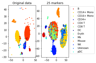
#TSNE plot
a=plot_marker_selection(data, markers, names)
Computing TSNE embedding
Elapsed time: 117.06255102157593 seconds
num_markers=25
method='pairwise'
sampling_rate=0.1 #use 10 percent of the data to generate constraints
n_neighbors=3 #3 constraints per point
epsilon=1 #Delta is 10*norm of the smallest constraint
max_constraints=1000 #use at most 1000 constraints (for efficiency)

markers= get_markers(data, labels, num_markers, method=method, sampling_rate=sampling_rate,
                     n_neighbors=n_neighbors, epsilon=epsilon, max_constraints=max_constraints)

accuracy=performance(data, labels, data, labels, clf)
accuracy_markers=performance(data[:,markers], labels, data[:,markers], labels, clf)

print("Accuracy (whole data,", d, " markers): ", accuracy)
print("Accuracy (selected", num_markers, "markers)", accuracy_markers)
Solving a linear program with 500 variables and 1000 constraints
Time elapsed: 6.737841844558716 seconds
Accuracy (whole data, 500 markers): 0.8660786816757572
Accuracy (selected 25 markers) 0.7710340025530927
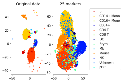
#TSNE plot
a=plot_marker_selection(data, markers, names)
Computing TSNE embedding
Elapsed time: 118.96086025238037 seconds